Learn TinyML using Wio Terminal and Arduino IDE #2 Audio Scene Recognition and Mobile Notifications
Updated on Feb 28th, 2024
It’s the second article of TinyML tutorials series and today I’ll teach you how to train and deploy an audio scene classifier with Wio Terminal and Edge Impulse. For more details and video tutorial, watch the corresponding video!
First some background about audio signal processing. If you want to jump straight to action, by all means, skip to the next section! Or not – I thought I already knew about sound processing, but while making this article I found out quite a few new things myself.
Sound processing for ML
Sound is an a vibration that propagates (or travels) as an acoustic wave, through a transmission medium such as a gas, liquid or solid.
The source of sound pushes the surrounding medium molecules, they push the molecules next to them and so on and so forth. When they reach other object it also vibrates slightly – we use that principle in microphone. The microphone membrane gets pushed inward by the medium molecules and then back to its original position.
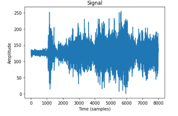
That generates alternating current in the circuit, where voltage is proportional to sound amplitude – the louder the sound, the more it pushes membrane, thus generating higher voltage. We then read this voltage with analog-to-digital converter and record at equal intervals – the number of times we take measurement of sound in one second is called a sampling rate, for example 8000 Hz sampling rate is taking measurement 8000 times per second. Sampling rate obviously matters a lot for quality of the sound – if we sample too slow we might miss important bits and pieces. The numbers used for recording sound digitally also matter – the larger range of a number used, the more “nuances” we can preserve from the original sound. That is called audio bit depth – you might have heard terms like 8-bit sound and 16 bit sound. Well, it is exactly what is says on the tin – for 8-bit sound an unsigned 8-bit integers are used, which has range from 0 to 255. For 16-bit sound a signed 16-bit integers are used, so that’s -32 768 to 32 767. Alright, so in the end we have a string of numbers, with larger numbers corresponding to loud parts of the sound and we can visualize it like this.
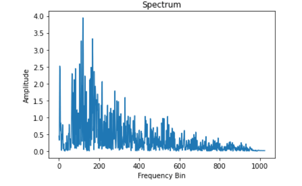
We can’t do much with this raw sound representation though – yes, we can cut and paste the parts or make it quilter or louder, but for analyzing the sound, it is, well, too raw. Here is where Fourier transform, Mel scale, spectrograms and cepstrum coefficients come in. There is a lot of materials on the Internet about Fourier transform, personally I really like this article from betterexplained.com and a video from 3Blue1Gray – check them out to find more about FFT. For purpose of this article, we’ll define Fourier transform as a mathematical transform, that that allows us to decompose a signal into it’s individual frequencies and the frequency’s amplitude.
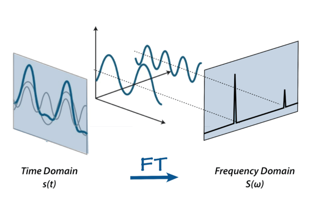
Or as it was put in betterexplained article – given the smoothie, it outputs the recipe. That is how our sound looks like after applying Fourier transform – the higher bars correspond to larger amplitude frequencies.
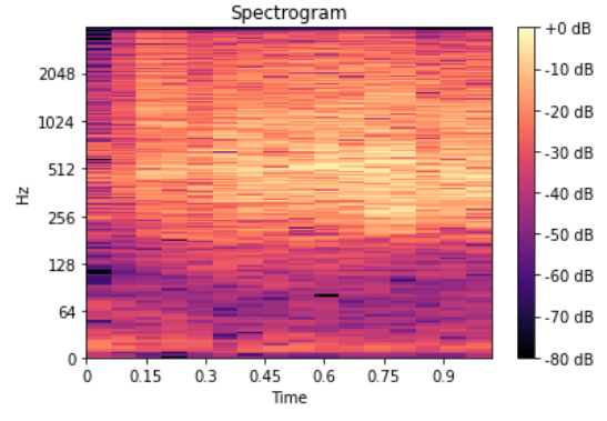
That’s great! Now we can do more interesting things with audio signal – for example eliminate the least important frequencies to compress the audio file or remove the noise or maybe the sound of voice, etc. But it is still not good enough for audio and speech recognition – by doing Fourier transform we loose all the time domain information, which is not good for non-periodic signals, such as human speech. We are smart cookies though and just take Fourier transform multiple times on the signal sample, essentially slicing it and then stitching the data from multiple Fourier transforms back together in form of spectrogram.
Here x-axis is the time, y-axis is frequency and the amplitude of a frequency is expressed through a color, brighter colors correspond to larger amplitude.
Very well! Can we do sound recognition now? No! Yes! Maybe!
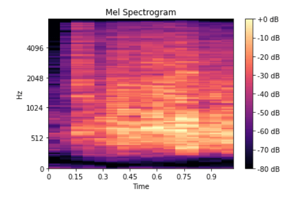
Normal spectrogram contains too much information if we only care about recognizing sounds that human ear can hear. Studies have shown that humans do not perceive frequencies on a linear scale. We are better at detecting differences in lower frequencies than higher frequencies. For example, we can easily tell the difference between 500 and 1000 Hz, but we will hardly be able to tell a difference between 10,000 and 10,500 Hz, even though the distance between the two pairs are the same.
In 1937, Stevens, Volkmann, and Newmann proposed a unit of pitch such that equal distances in pitch sounded equally distant to the listener. This is called the mel scale.
A mel spectrogram is a spectrogram where the frequencies are converted to the mel scale.
There are more steps involved for recognizing speech – for example cepstrum coefficients, that I mentioned above – we will discuss them in later videos of the series. It is time to finally start with practical implementation.
Collect the training data
In the last video of the series we used data-forwarder tool of edge-impulse-cli to gather the data (see how to install it in the first article of the series). Unfortunately we cannot do the same for audio signal, since data-forwarder has maximum signal frequency capped at 370 Hz – way too low for audio signal. Instead download a new version of Wio Terminal Edge Impulse firmware with microphone support and flash it to your device. After that create a new project on Edge Impulse platform, launch edge-impulse ingestion service
edge-impulse-daemon
Then log in with your credentials and choose a project you have just created. Go to Data Acquisition tab and you can start getting data samples. We have 4 classes of data and will record 10 samples for each class, 3000 milliseconds duration each. I’ll be recording the sounds played from the laptop (except for background class), if you have the opportunity to record real sounds, that would be even better. 40 samples is abysmally small, so we’re also going to upload some more data. I simply downloaded the sounds from YouTube, resampled them to 8000 Hz and saved them to .wav format with simple converter script – you’ll need to install librosa with pip to run it.
import librosa
import sys
import soundfile as sf

input_filename = sys.argv[1]
output_filename = sys.argv[2]

data, samplerate = librosa.load(input_filename, sr=8000) # Downsample 44.1kHz to 8kHz
print(data.shape, samplerate)

sf.write(output_filename, data, samplerate, subtype='PCM_16')
Then I cut all the sound samples to leave only “interesting” pieces – I did that for every class, except for background.
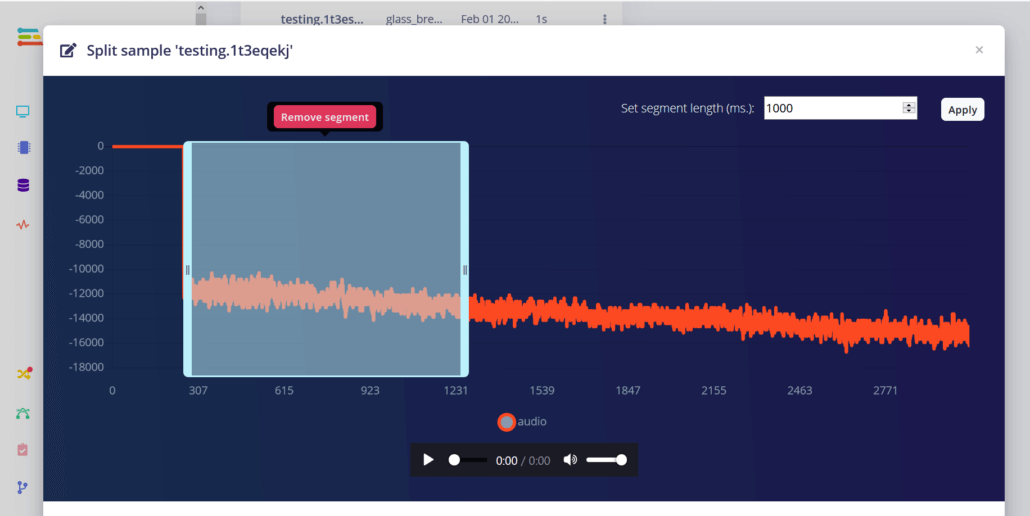
After the data collection is done, it is time to choose processing blocks and define our neural network model.
Data processing and Model training
Among the processing blocks we see three familiar options – namely Raw, Spectral Analysis, which is essentially Fourier transform of the signal, Spectrogram and MFE (Mel-Frequency Energy banks) – which correspond to four stages of audio processing I described earlier!
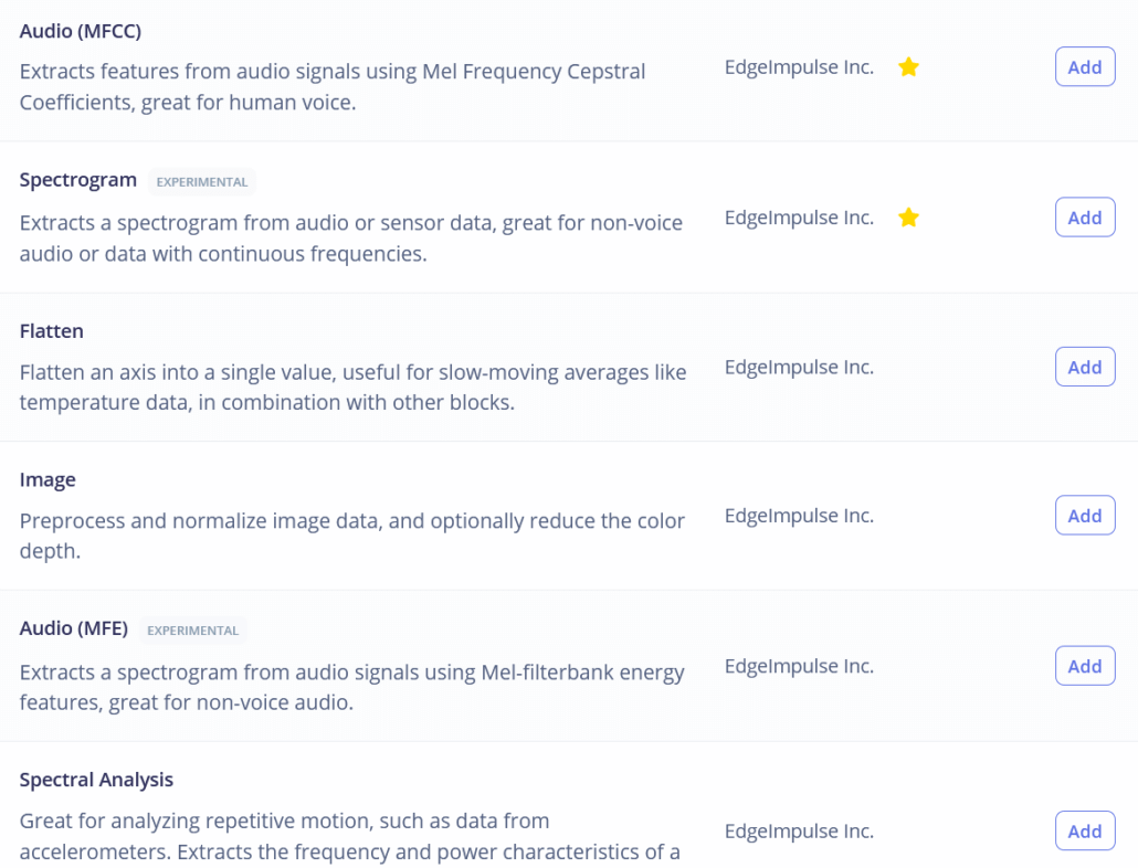
If you like experimenting, you can try using all of them on your data, except for maybe Raw, which will have too much data for our small-ish neural network. I’ll just go with the best option for this task, which is MFE or Mel-Frequency Energy banks. After computing the features, go to NN classifier tab and choose a suitable model architecture. The two choices we have are using 1D Conv and 2D Conv. Both will work, but If possible, we should always go for smaller model, since we will want to deploy it to embedded device. I ran 4 different experiments, 1D Conv/2D Conv with MFE and MFCC features and the results for them are in this table. The best model was 1D Conv network with MFE processing block. By tweaking MFE parameters (namely increasing stride to 0.02 and decreasing low frequency to 0) I increased accuracy from 75 % for default parameters to 85 % on the same dataset.
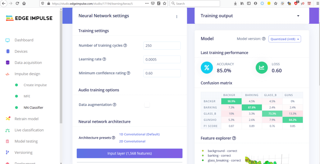
You can find the trained model here and test it out yourself. While it is good at distinguishing barking and gunshots from background, glass breaking sound detection accuracy was fairly low during live classification and on-device testing. I suspect this is due to 8000 Hz sampling rate – the highest frequency that is present in recording is 4000 Hz and glass breaking has a lot of high-pitched noise, that could help distinguishing this particular class from the others.
Deployment
After we have our model and satisfied with its accuracy in training, we can test it on new data in Live classification tab and then Deploy it to Wio terminal. We’ll download it as Arduino library, put it in Arduino libraries folder and open microphone inference demo. The demo is based on Arduino Nano 33 BLE and uses PDM library. Because of Wio Terminal relatively simple microphone circuit and to keep things really simple this time, we will just use analogRead function and delayMicroseconds for timing.
static bool microphone_inference_record(void)
{
    inference.buf_ready = 0;
    inference.buf_count = 0;

    if (inference.buf_ready == 0) {
        for(int i = 0; i < 8001; i++) {
            inference.buffer[inference.buf_count++] = map(analogRead(WIO_MIC), 0, 1023, -32768, 32767);
            delayMicroseconds(sampling_period_us);

            if(inference.buf_count >= inference.n_samples) {
                inference.buf_count = 0;
                inference.buf_ready = 1;
                break;
            }
        }
    }

    return true;
}
A large disclaimer here – that is not the way how to properly record sound. Normally we would use interrupts to time the audio sampling, but interrupts is a large topic by itself and I want you to finish this video before you get old. So, we’ll leave that (together with MFCC explanation) for later article about speech recognition.
After uploading the sample code, which you can find in this Github repository, open the Serial monitor and you will see probabilities for every classes printed out. Play some sounds or make your dog bark to check the accuracy! Or watch the demo in the video above.
Mobile notifications with Blynk
It works great, but not very practical – I mean if you can see the screen, then you probably can hear the sound yourself. Since Wio Terminal can connect to the Internet, we can take this simple demo and make it into a real IoT application with Blynk.
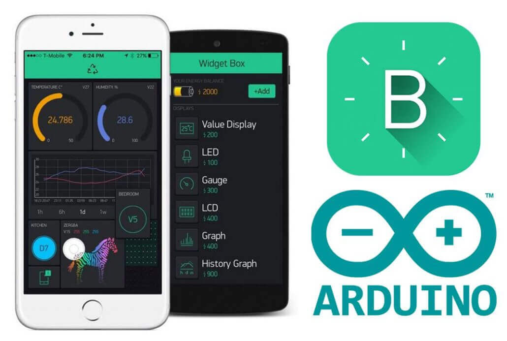
Blynk is a platform that allows you to quickly build interfaces for controlling and monitoring your hardware projects from your iOS and Android devices. In this case we will use Blink to push notification to our phone if Wio Terminal detects any sounds we should worry about.
To get started with Blink, download the app, register a new account and create a new project. Add a push notification element to it and press play button. For Wio terminal, install Seeed_Arduino_rpcWiFi, Seeed_Arduino_rpcUnified, Seeed_Arduino_mbedtls and Seeed_Arduino_FS libraries. Then try Blynk with simple push button example – make sure you change WiFi SSID, password and your Blynk API token.
#define BLYNK_PRINT Serial

#include <rpcWiFi.h>
#include <WiFiClient.h>
#include <BlynkSimpleWioTerminal.h>

char auth[] = "token";
char ssid[] = "ssid";
char pass[] = "password";

void checkPin()
{
  int isButtonPressed = !digitalRead(WIO_KEY_A);
  if (isButtonPressed) {
    Serial.println("Button is pressed.");
    Blynk.notify("Yaaay... button is pressed!");
  }
}

void setup()

{
  Serial.begin(115200);
  Blynk.begin(auth, ssid, pass);
  pinMode(WIO_KEY_A, INPUT_PULLUP);
}

void loop()
{
  Blynk.run();
  checkPin();
}
If code compiles and the test is successful (pressing top left button on Wio Terminal causes a push notification to appear on your phone), then we can move to the next stage.
We’re going to move all the neural network inference code in a separate function and call it in the loop() function right after Blynk.run(). Similar to what we did before, we check the neural network prediction probabilities and if they are higher than threshold for a certain class, we call Blynk.notify() function, which as you might have guessed pushes a notification to your mobile device. Find the full code for NN inference + Blynk notification here.
And voila, we have a working ML on the Edge IoT application, that can be used to warn people about dangerous situations! There are few things that can be – and will be improved, most importantly, continuous sound sampling for inference and higher sampling rate to increase sound quality.
Try it our on your own set of sounds. If you do, post your feedback in the video or article comments! Stay tuned for more articles!
Choose the best tool for your TinyML project
Grove – Vision AI Module V2
It’s an MCU-based vision AI module powered by Himax WiseEye2 HX6538 processor, featuring rm Cortex-M55 and Ethos-U55. It integrates Arm Helium technology, which is finely optimized for vector data processing, enables:
- Award-winning low power consumption
- Significant uplift in DSP and ML capabilities
- Designed for battery-powered endpoint AI applications
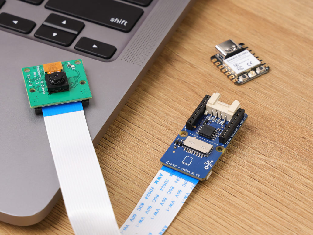
With support for Tensorflow and Pytorch frameworks, it allows users to deploy both off-the-shelf and custom AI models from Seeed Studio SenseCraft AI. Additionally, the module features a range of interfaces, including IIC, UART, SPI, and Type-C, allowing easy integration with popular products like Seeed Studio XIAO, Grove, Raspberry Pi, BeagleBoard, and ESP-based products for further development.
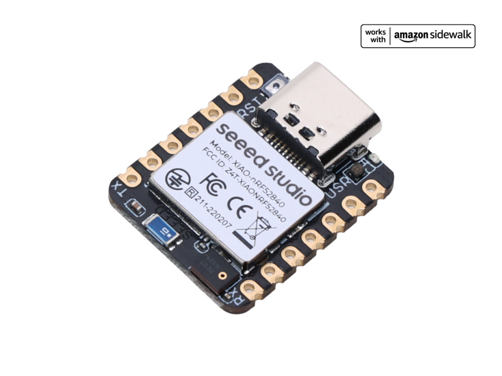
Seeed Studio XIAO ESP32S3 Sense & Seeed Studio XIAO nRF52840 Sense
Seeed Studio XIAO Series are diminutive development boards, sharing a similar hardware structure, where the size is literally thumb-sized. The code name “XIAO” here represents its half feature “Tiny”, and the other half will be “Puissant”.
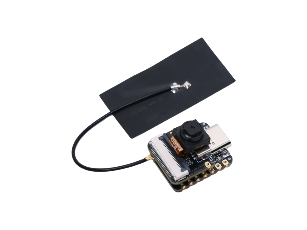
Seeed Studio XIAO ESP32S3 Sense integrates an OV2640 camera sensor, digital microphone, and SD card support. Combining embedded ML computing power and photography capability, this development board can be your great tool to get started with intelligent voice and vision AI.
Seeed Studio XIAO nRF52840 Sense is carrying Bluetooth 5.0 wireless capability and is able to operate with low power consumption. Featuring onboard IMU and PDM, it can be your best tool for embedded Machine Learning projects.
Click here to learn more about the XIAO family!
SenseCraft AI
SenseCraft AI is a platform that enables easy AI model training and deployment with no-code/low-code. It supports Seeed products natively, ensuring complete adaptability of the trained models to Seeed products. Moreover, deploying models through this platform offers immediate visualization of identification results on the website, enabling prompt assessment of model performance.
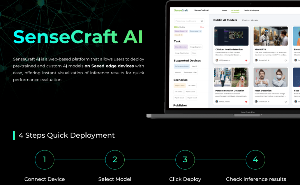
Ideal for tinyML applications, it allows you to effortlessly deploy off-the-shelf or custom AI models by connecting the device, selecting a model, and viewing identification results.
References and sources
Understanding the Mel Spectrogram
Why do Mel-filterbank energies outperform MFCCs for speech commands recognition using CNN?