Mobile Robot Full-stack Development In Practice Ⅱ: Give the Robot Its Eyes — GMSL2 Multi-Camera, Calibration, and BEV Surround View

If this is your first time coming across the series, Mobile Robot Full-stack Development In Practice is an open-source, hands-on course built around a simple idea: instead of learning robotics as a collection of isolated algorithms, learn how the pieces connect into a real system.

In the first article, we built the robot’s computing and development foundation — a Jetson-powered reComputer Robotics J501, a validated JetPack environment, remote development, and ROS 2 communication between the robot and a host PC. That foundation is what makes this article possible. It is also exactly what a robot needs before it can perceive anything.

The course now moves from the computing platform into perception, sensor fusion, SLAM, autonomous navigation, semantic understanding, manipulation, and deployment.

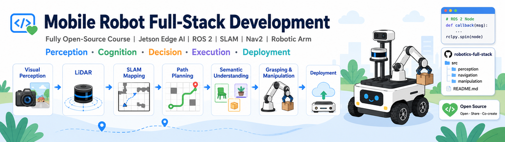
If you have not seen the full course overview yet, start there first to understand the overall learning path.

👉 Course Introduction

👉 Mobile Robot Full-Stack Development GitHub

👉 M02 — Fundamentals of Vision Systems

When you actually put four cameras on a mobile robot, the first problem is rarely “which detection model should I run?” A more basic set of questions comes first. Does the image data reliably reach the computer? Do four sensors expose at the same instant? If the robot is turning while the cameras are capturing, how should those images be combined? And how much of the resulting picture is something the robot actually observed, rather than something the renderer filled in for appearance?

If that geometry is missing, even a strong perception model or a well-tuned stitching pipeline can remain nothing more than an attractive demo.

So this second article focuses on something less flashy, but much more fundamental:

How does a robot turn several camera streams into spatial information with known geometry, timing, and validity?

Each fisheye lens has its own field of view and imaging behaviour, so the same ground target appears at a different pixel position in every image. Differences in lens distortion, mounting angle, and capture time introduce further misalignment. If you want to unify four directional images into a single bird’s-eye view with a real spatial scale, you must first solve image transmission, camera synchronization, geometric calibration, and multi-view stitching. Getting from four independent video streams to one trustworthy surround view is exactly the technical chain this article breaks down.

The reference setup used here is a reComputer Robotics J501 with its GMSL expansion solution and GMSL2 cameras such as the SG3S-ISX031C-GMSL2F, plus four roughly 198° fisheye lenses for the surround-view work, running ROS 2 Humble on Ubuntu 22.04 with a host PC used for development and validation.

Four Cameras Are Not Simply Four Video Streams

Moving from a single USB camera for a vision demo to four cameras mounted around a mobile robot adds far more than image count. Longer cables mean video must stay stable next to motors and power wiring. The camera fields of view must cover the different directions around the vehicle. More importantly, while the robot is moving, different cameras must observe the environment as close to the same moment as possible. If one camera exposes first and another a little later, the vehicle has already translated or rotated, and even precise geometric calibration will not prevent a stitching misalignment.

GMSL2 (Gigabit Multimedia Serial Link 2) is a high-speed serializer/deserializer technology designed for exactly these automotive and high-reliability scenarios. In a typical link, the image sensor’s CSI-2 data enters a serializer, travels over a coaxial or shielded twisted-pair cable, and is recovered as CSI-2 by a deserializer near the computing platform. The link can also carry reverse control signals, and power can be delivered over the cable (PoC) to simplify wiring. CSI-2 is responsible for how image data enters the processor; GMSL2 is responsible for carrying that data reliably across a longer physical distance. The two usually work together rather than being a choice between them.

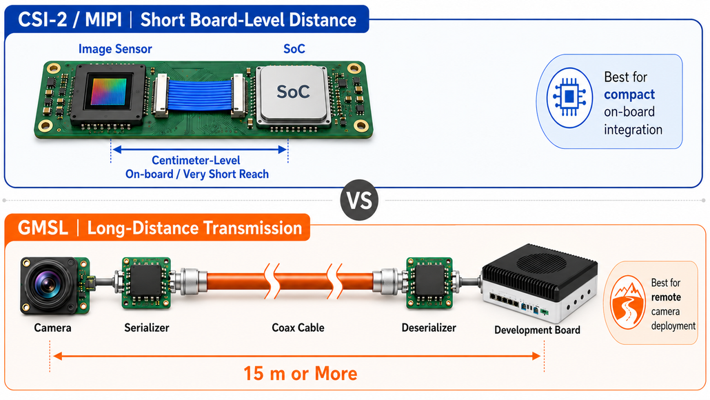
One point needs to be made explicit: the J501, expansion board, and cameras are not identical across every section of this module, and the 1920×1536 / sensor_mode=0 settings belong to the SG3S example rather than to every GMSL camera. Before wiring anything up, select the device tree and sensor mode that match your own hardware combination. The device tree tells Linux how the camera is connected; choose the wrong one and, even with intact hardware, the system may fail to create a working capture channel.

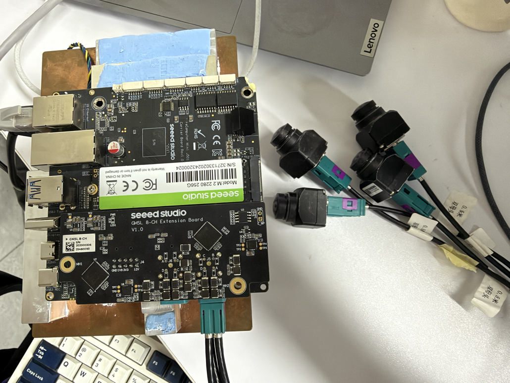
The board in this setup is the reComputer Robotics J501 carrier family — an AGX Orin platform with an 8-channel GMSL2 expansion board (MAX96712 deserializer) feeding MIPI CSI-2, which is the same hardware path used for BEV, occupancy-grid, and multi-camera SLAM workloads.

Two configurations are available:​
👉 reComputer Robotics J5011 with GMSL — Jetson AGX Orin 32GB, up to 200 TOPS
👉 reComputer Robotics J5012 with GMSL — Jetson AGX Orin 64GB, up to 275 TOPS

Before OpenCV or ROS 2: Verify the Linux Media Pipeline

When something actually fails, do not start by running a detection program. First check whether the system has created the video devices, and whether the media link between serializer, deserializer, CSI, and V4L2 has been established. This may look basic, but it reflects one of the most important debugging habits in robotics: verify the physical and operating-system layer before debugging the application layer. Reinstalling ROS 2 will not fix a camera that was never detected.

# Verify that V4L2 camera nodes exist
ls /dev/video*

# Inspect sensor → serializer → deserializer → CSI → V4L2 entities
media-ctl -d /dev/media0 -p

# Check whether another process has opened the camera nodes
fuser /dev/video0 /dev/video1 /dev/video2 /dev/video3

The division of labour is clear: ls confirms whether the device nodes exist, media-ctl shows the media entities and their relationships, and fuser reveals whether a camera is already held by a calibration program, a preview script, or another process.

For the four SG3S cameras in the tutorial, you must also confirm the pixel format and resolution, for example YUYV at 1920×1536 with the matching sensor_mode=0. If you switch to 1920×1080 or a different camera model, this set of parameters cannot be copied blindly. Rather than stacking every media-ctl --set-v4l2 command into the article, the more important judgement during real development is this: the device tree, the media entity formats, the V4L2 output format, and the camera’s actual mode must be one consistent combination. The complete setup commands and model tables are in the GMSL2 camera integration experiment in the M02 documentation.

# Inspect the format currently configured on all four cameras
for i in 0 1 2 3; do
  echo "===== /dev/video${i} ====="
  v4l2-ctl -d /dev/video${i} --get-fmt-video --get-parm
done

Camera Synchronization Is More Than Starting Multiple Processes

Multi-camera synchronization involves a deeper distinction: starting four capture processes at the same time does not mean the four sensors expose at the same instant. The GMSL configuration for the J501 passes an FSYNC signal through the MAX96712 deserializer and the MAX96717 serializers so that a unified cadence can reach the trigger inputs of multiple sensors. This is the basis for hardware synchronization. But the fact that the hardware can synchronize does not mean every downstream software node pairs frames strictly by timestamp; the current real-time surround-view renderer uses the latest frame from each camera, so motion can still produce brief seam misalignment because of the time difference. Understanding these two layers is what lets you judge correctly how far a multi-camera system has actually been verified.

The repository provides gmsl4_start.sh, with modes including preview, stream, verify, stop, and status. Before running it you need to deploy the script to the Jetson and check the resolution and frame rate against your specific camera. Use preview when a display is available, and verify first on a headless device to confirm the capture link, rather than treating the script as a plug-and-play command for arbitrary hardware.

# Prerequisites: camera-specific device tree, formats, and script deployment
bash ~/gmsl4_start.sh preview

# Headless verification
bash ~/gmsl4_start.sh verify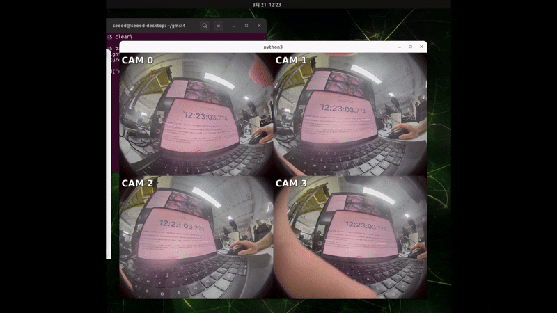

At this point, the robot can reliably capture images from several directions. But these are still two-dimensional pixels. To judge obstacle distance, recover object shape, and perform spatial fusion, you have to answer another question: where in the three-dimensional world does each pixel actually fall?

Once the four GMSL2 cameras output frames reliably, the robot has the basis for observing its surroundings. Those frames still have their own viewpoints, lens distortion, and coordinate frames, so even when they image the same patch of ground, objects appear at different pixel positions. Stitching them directly would leave ground lines unable to line up, and the same object could appear displaced or doubled at a seam. Converting four fisheye images into a unified bird’s-eye view starts by establishing how each camera forms an image, and where it sits relative to the robot chassis. That leads to the most important step in a multi-camera vision system: camera calibration.

Alongside multi-camera surround view, M02 also provides a separate RGB-D depth camera and 3D point-cloud exercise, covering depth-sensing principles, Gemini 2 integration, depth-to-color alignment, and point-cloud generation. If that part interests you, go to the complete M02 documentation on GitHub, open Section 2.2 Depth Cameras and 3D Visual Perception, and work through it with the code.

Camera Calibration: Turning Pixels into Spatial Measurements

The four GMSL2 cameras now output frames reliably, but their lens distortion, mounting positions, and orientations all differ, so they cannot be stitched directly into an accurate surround view. Mapping views from different angles into one common ground coordinate frame requires calibration: intrinsics, distortion parameters, and extrinsics relative to the robot chassis. These form the geometric foundation for everything that follows — fisheye undistortion, perspective transforms, and BEV stitching.

For the ideal pinhole model, a spatial point ((X_c,Y_c,Z_c)) projected onto the normalized plane satisfies (x=X_c/Z_c) and (y=Y_c/Z_c). The intrinsic matrix (K) then converts normalized coordinates into pixel coordinates:

[ K=\begin{bmatrix}f_x&0&c_x\0&f_y&c_y\0&0&1\end{bmatrix} ]

Here (f_x,f_y) are the equivalent focal lengths in pixels and ((c_x,c_y)) is the principal point. Real lenses also introduce radial and tangential distortion, described by a model and distortion coefficients (D). When the robot needs to know a camera’s orientation and position relative to the vehicle, it also needs the extrinsic rotation (R) and translation (t). If (P_w) is a point in the reference frame, then (P_c=RP_w+t); here the direction of the transform and the reference frame must be stated clearly, because a matrix that looks correct can still project objects to an entirely wrong position.

Calibration works by using the corner positions that are genuinely known on the calibration board and the corner positions detected in the image, and solving backwards for (K,D,R,t) so that the model’s predicted pixels land as close as possible to the actual detections. The error is usually described by the reprojection RMS:

[ e_{\mathrm{RMS}}=\sqrt{\frac1N\sum_{i=1}^{N}\lVert\hat p_i-p_i\rVert^2} ]

A smaller error does not automatically mean the calibration is reliable for every downstream task. If dozens of calibration photographs are taken at the same distance and the same tilt, the geometric constraints they provide are still very limited. High-quality capture means moving the chessboard through the centre and the edges of the image, varying distance and pose, while avoiding blur, reflections, focus changes, and paper deformation. For ordinary perspective lenses, an RMS of around one pixel can serve as an initial reference, but it must not be treated as a universal pass/fail line for all resolutions, fisheye lenses, and high-precision tasks.

The introductory perspective-camera example uses a board with 9×7 squares, which means 8×6 inner corners. In the following command, 0.020 represents the case where the actually measured square width is 20 mm. --size is the number of inner corners and --square is the real side length of one square; the two parameters must not be confused. The full procedure requires the camera driver to be publishing the corresponding image_raw topic first, and after calibration the resulting camera_info YAML must be saved and loaded.

# Prerequisites: ROS 2 and a camera driver publishing the image topic
sudo apt install ros-humble-camera-calibration

ros2 run camera_calibration cameracalibrator \
  --no-service-check --size 8x6 --square 0.020 \
  --ros-args -r image:=/gmsl/cam0/image_raw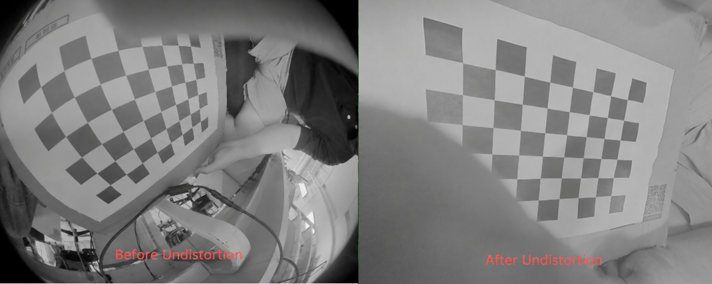

For stereo cameras, calibration also requires that the left and right images come from corresponding moments in time, and it solves for the rotation and translation between the two cameras. Epipolar rectification then follows, so that the same point in space falls as close as possible on the same image row in both images, reducing the search for corresponding points from a two-dimensional area to a one-dimensional search along a scanline. The usable outputs here are not only the before-and-after screenshots, but also the parameter files, the error report, and the row-alignment result for the corresponding points. Only when these results can be loaded and verified by the downstream driver has the calibration become a real engineering asset.

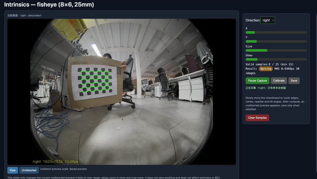
The four roughly 198° fisheye cameras are a different case. The plumb_bob model commonly used for ordinary perspective cameras should not be applied directly to describe a lens with such a large field of view, and the advanced practice uses the equidistant route through cv2.fisheye.calibrate. The calibration data must cover different X/Y/Size/Skew values, rather than repeatedly shooting from the same pose to pad the frame count. The balance parameter of undistortion changes the new camera matrix and the preserved field of view, so a ground mapping solved previously under one set of (K,D,balance) cannot continue to be reused unconditionally after those parameters change.

The four-fisheye calibration uses a different chessboard: 8×6 inner corners with 25 mm squares. This must not be mixed up with the 20 mm ordinary calibration example above. After the camera driver and calibration packages are deployed, stop the capture programs that occupy the cameras before starting the Web calibration console. Enter /intrinsics to solve the intrinsics one camera at a time, check the undistortion preview and the quality report, then enter /extrinsics to measure the chessboard’s position relative to the vehicle and solve for the extrinsics. The /bev page in the browser is only a stitching preview and cannot replace the real ROS 2 metric BEV acceptance in the next stage.

# Prerequisites: j501_avm_calib and scripts/run_calib_web.sh deployed per the repository
# This console owns the V4L2 devices; stop the camera driver / real-time BEV first
cd ~/workspace/ros2_bev
bash scripts/run_calib_web.sh

Open http://<Jetson_IP>:8090 in the host PC browser and complete /intrinsics, then /extrinsics (checking /seam if needed). Four intrinsics JSON files, one extrinsics.json, and four YAML files with distortion_model: equidistant should all exist before the BEV stage has its inputs. If the intrinsics are re-solved, the old extrinsics may be marked as stale and must be recalibrated; the previous ground mapping cannot be forced to keep working.

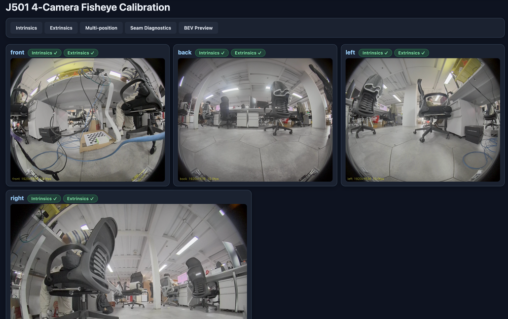
There is one engineering detail here that easily produces an “image appears on the wrong side” result: the ground coordinate convention inside the four-fisheye calibration tool is +X right, +Y forward, +Z up, while the common ROS REP-103 body convention is +X forward, +Y left, +Z up. When connecting other ROS modules or TF, you must define the axis mapping explicitly instead of treating two sets of coordinate values as the same notation. At the same time, the corner ordering when the chessboard is rotated 180° is ambiguous. If one camera’s view is flipped to the other side of the vehicle, check the chessboard orientation and the ground-point correspondence first, rather than immediately redoing all the intrinsics.

From Four Fisheye Views to One Metric Bird’s-Eye View

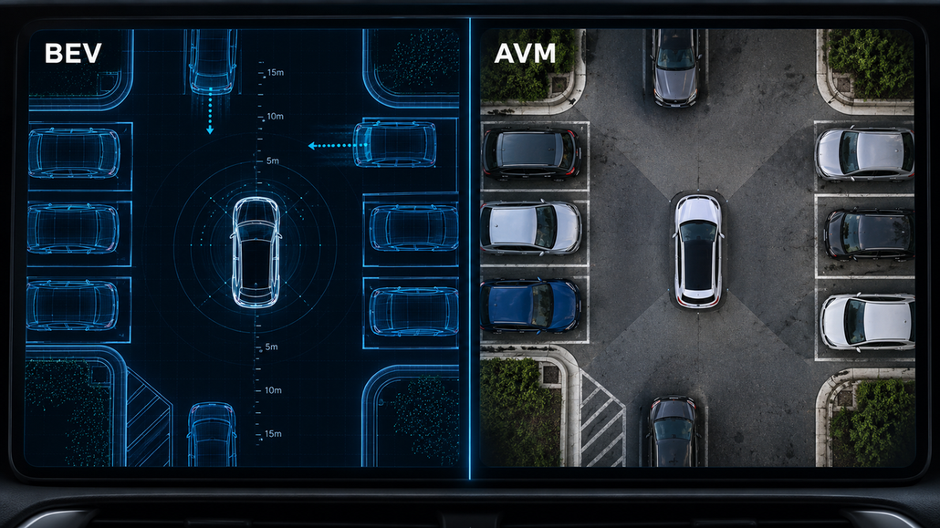
Once all four fisheye cameras are calibrated, we know how each camera forms an image and where it is mounted. The remaining problem is how to place the ground they each see into one image. BEV uses the approximation that the ground is a plane, turning a perspective view into a representation centred on the robot with a consistent ground scale. This is different from an ordinary photo collage: the four images do not only need their edges to line up. Every final pixel should have a clear spatial meaning, and you need to know whether it was actually observed by a camera.

The core tool here is the homography matrix (H). If we define (H) as the mapping from ground coordinates to image coordinates, then a point ((X,Y)) on the plane and the camera pixel ((u,v)) satisfy:

[ s\begin{bmatrix}u\v\1\end{bmatrix}=H\begin{bmatrix}X\Y\1\end{bmatrix} ]

This is a projective relationship, and the overall scale of the matrix does not affect the final projection. In the pinhole model, taking the ground as (Z=0) yields the corresponding plane relationship from ((K,R,t)); the actual four-fisheye calibration chain instead solves the mapping directly from the real placement of the ground chessboard and corner detection. Note that the (H) saved in the tutorial is bound to the undistorted image and the calibration canvas, and at runtime it must be combined with the view transform and an appropriate inverse. You cannot assume that two matrices both named H point in the same direction simply because another tutorial also writes down an H.

One counter-intuitive but important implementation question: why not project every pixel of the fisheye image directly “onto” the bird’s-eye view? Forward projection brings holes, repeated writes, and sampling conflicts. A more reliable approach is to search backwards — for each pixel on the BEV canvas, first work out which ground position it represents, and then find where its colour should be sampled in the original fisheye image. This is what inverse perspective mapping (IPM) means here.

Taking the tutorial’s default 600×600 canvas covering 4×4 metres of ground as an example, the scale is about 150 pixels per metre. Each BEV pixel is first converted to a ground coordinate, then mapped through the calibration and view transform to the undistorted image, the normalized ray is recovered with the new intrinsics, and finally the fisheye distortion model gives the sampling coordinate in the raw image. The chain can be summarized as:

BEV pixel → ground position → undistorted pixel → normalized camera ray → raw fisheye pixel

The renderer precomputes these sampling relations into mapx / mapy and uses cv2.remap lookups during live operation, avoiding a full re-solve of the geometry on every frame.

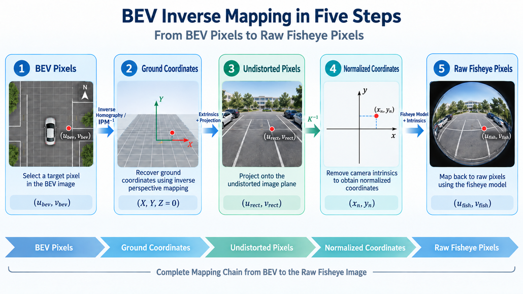
But the fact that inverse mapping can find a sampling location does not mean that this piece of ground can actually be seen by a camera. The sampling point may lie outside the raw image, may come from the wrong branch after the homography is extended, or may be extrapolated beyond the camera’s viewing sector. The renderer therefore performs an in-bounds check, a valid-ground-branch check, and an angular sector check in order. Only when all these conditions are met does a pixel have real camera observation behind it; the valid support of all cameras combined forms /avm/bev/valid_mask.

The most important engineering principle here is that unknown areas must remain unknown. For a human-facing surround view, blank areas may affect the visual result. But in a bird’s-eye view with a real spatial scale, a position that no camera actually observed cannot be treated as confirmed free ground. A surround view made for people may soften the gaps for appearance, but a map genuinely used for local spatial reasoning must never paint unobserved areas as known ground. Otherwise a downstream system may mistake a position the robot never saw for verified navigable space. In this project, /avm/bev/metric/image is the image that carries ground scale and must be used together with valid_mask; /avm/bev/surround/image is the surround or bowl-style picture for human observation and must not be used as a ruler. Additional outputs describe camera ownership and rendering diagnostics. This matters because a view optimized for easy observation is not automatically a valid measurement surface for localization or navigation.

Why Wide-Area Blending Produces Ghosting

The four fisheye views overlap each other, and the seams introduce a new contradiction: if the same object in adjacent views differs by only a few pixels, blending over a large area can produce double images. The renderer therefore uses a hard-first, soft-second strategy: it first assigns each pixel a primary camera, and then applies a narrow transition band only near the ownership boundary. Brightness gains are estimated from the overlap region to compensate for exposure differences between the four cameras, and seam refinement can, when needed, adjust the boundary along a path where the image difference is smaller. The default transition band is about 4 cm (transition_m=0.04); it is not a best value that every scenario must copy, but a practical compromise between a smooth boundary and avoiding ghosting.

Running and Validating the Real-Time Renderer

Before running the real-time BEV, the four-fisheye calibration must be complete, and the four JSON files, the extrinsics, and the equidistant YAML files must be checked. avm_ros2 also depends on the j501_avm_calib camera driver deployed earlier. The Web calibration console and the camera driver contend for the same V4L2 devices, so the calibration program should be stopped before the real-time renderer starts. The key build and run commands are kept below; the complete package deployment, file paths, and launch parameters are still defined by the M02 BEV experiment documentation.

# Prerequisites: j501_avm_calib deployed, four sets of calibration files ready
cd ~/workspace/ros2_bev/ros2_ws
source /opt/ros/humble/setup.bash
source ~/ros2_ws/install/setup.bash
colcon build --packages-select avm_ros2 --symlink-install
source install/setup.bash

# Stop the Web console before the driver opens V4L2 devices
pkill -f calib_web.py || true

ros2 launch avm_ros2 avm_rviz.launch.py \
  start_camera_driver:=true

After starting, besides viewing the stitching result in RViz2, you should verify that the metric bird’s-eye view and the valid mask publish continuously, that all four cameras are online, and that the diagnostics are healthy. The default canvas is 600×600 covering 4×4 metres, with a target render rate of 5 Hz. With require_all_cameras=true, any single camera dropping out or timing out can prevent the complete image from publishing. At that point, check the camera topics one by one before considering disabling that requirement for diagnosis — there is no need to redo the entire calibration immediately.

ros2 topic list | grep /avm/bev
ros2 topic hz /avm/bev/metric/image
ros2 topic info /avm/bev/valid_mask
ros2 topic echo /avm/bev/diagnostics --once

Finally, the boundaries of this BEV need to be kept in view. The homography projection here is built on the assumption that the ground is approximately planar, so ground lines and the contact points of objects have geometric reference value, while the upper halves of a standing person, a chair, or a box may be stretched in the bird’s-eye view. Ground slope, changes in the camera mount, exposure differences, and taking the latest frame from multiple cameras during motion all affect the result. BEV is one way to represent ground space reliably; it is not a way to turn four views directly into a complete three-dimensional world.

What You Should Remember Is the Debugging Order

If you only want to get the four cameras running, you can copy the commands and move on.

If you want this article to remain useful months later, keep the debugging order instead.

If a camera produces no image, do not immediately reinstall ROS 2. Check the device tree, the V4L2 nodes, and the media graph first, then look for processes already holding the devices. If frames are misaligned during motion, check camera synchronization and the timing relationship rather than widening the blending region. If fisheye undistortion looks wrong near the edges, verify the camera model and the sample diversity, because a plumb_bob model on a 198° lens fails quietly.

The whole chain can be summarized as:

Hardware connection → Time synchronization → Camera calibration → Coordinate transformation → BEV projection and fusion

Lower layers should usually be ruled out first, and a BEV seam displacement should send you back to ground placement, corner orientation, and extrinsics rather than to a wider blend.

That habit is far more valuable than memorizing every command in the tutorial.

By the end of this module, the result is not simply “four cameras that display images.”

It is a vision system that is ready to feed the next stage:

• four camera streams are verified and format-consistent;
• the hardware and software timing layers are understood as two separate things;
• intrinsics, extrinsics, and their coordinate conventions are explicit;
• the surround view distinguishes observed ground from unobserved ground;
• the metric output is validated together with its valid mask.

The most important principle is that a complete picture does not mean accurate geometry, and areas not observed by a camera cannot be treated as known ground.

The next article moves into LiDAR and multi-sensor fusion. The question changes from:

“How does the robot begin to see the world?”

to:

“How does the robot know where it is, and where it is going?”

That means LiDAR, IMU, GNSS/GPS, and CAN-FD, the time and spatial alignment between them, and EKF-based state estimation.

Build Along and Share What You Learn

Mobile Robot Full-stack Development In Practice is an open-source series, and we want it to become more than a sequence of tutorials.

If you reproduce the setup and encounter a different result, find a better configuration, integrate another sensor, or build your own demo on top of the platform, share it.

You do not need to wait until you have built a complete autonomous robot. Your first four-camera preview, your first correctly aligned calibration, or even a seam problem you cannot solve are all useful starting points for discussion.

The global Seeed Studio robotics community is open to developers who want to share demos, compare setups, discuss what they are learning, ask practical questions, and connect directly with Seeed Studio developers and engineers.

Join the community:

• Seeed Studio Discord
• WhatsApp Robotics Discussion Group
• Facebook AI Robotics Community Group
• Course GitHub ⭐ & Fork it

Build something small. Share what worked. Share what broke. Help someone else reproduce it.

That is how an open robotics course becomes an open robotics community.

Resources Used in This Article

Hardware

reComputer Robotics J501 Series with GMSL expansion solution

SG3S-ISX031C-GMSL2F GMSL2 cameras ×4

Fisheye lenses (approximately 198°) for the surround-view experiment

Mini-Fakra coaxial cable

Software Stack

ROS 2 Humble

V4L2 / media-ctl (V4L2 media graph)

OpenCV (fisheye calibration model, remap)

reComputer Robotics J501 hardware guide

Hands-on Documentation

M02 — Fundamentals of Vision Systems

Orbbec ROS 2 driver documentation — for the separate depth-camera exercise in Section 2.2

About Author

Frank

See author's posts